Suppose that Y1,…,Yn are independent observations, with Yi having probability density function of the following form
f(yi∣θi,ϕ)=exp[ϕyiθi−b(θi)+c(yi,ϕ)]
where E(Yi)=μi and g(μi)=βTxi. You should assume that g() is a known function, and β,ϕ are unknown parameters, with ϕ>0, and also x1,…,xn are given linearly independent covariate vectors. Show that
∂β∂ℓ=∑g′(μi)Vi(yi−βi)xi
where ℓ is the log-likelihood and Vi=var(Yi)=ϕb′′(θi).
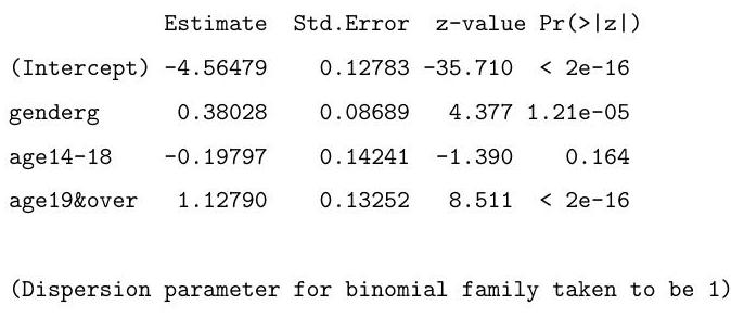
Discuss carefully the (slightly edited) R output given below, and briefly suggest another possible method of analysis using the function glm ( ).
>s<−scan()
1: 336315738108159
7:
Read 6 items
>r<−scan()
1: 327172565065248688773520
7:
Read 6 items
> gender <- scan(,"∥)
1: b b b g g g
7:
Read 6 items
> age <- scan(,"′)
1: 13&under 14-18 19&over
4: 13&under 14-18 19&over
7 :
Read 6 items
> gender <- factor (gender) ; age <- factor (age)
>summary(glm(s/r∼ gender + age, binomial, weights =r))
Coefficients:

Null deviance: 221.797542 on 5 degrees of freedom
Residual deviance: 0.098749 on 2 degrees of freedom
Number of Fisher Scoring iterations: 3
