Consider performing a two-way analysis of variance (ANOVA) on the following data: >Y[,,1] Y[,,2] Y[,,3] [,1][,2] [,1][,2] [,1][,2]

Explain and interpret the R commands and (slightly abbreviated) output below. In particular, you should describe the model being fitted, and comment on the hypothesis tests which are performed under the summary and anova commands. >K<−dim(Y)[1] >I<−dim(Y)[2] >J<−dim(Y)[3] >C(I,J,K)
[1] 2310
>y<− as.vector (Y)
>a<−gl(I,K, length (y))
>b<−gl(J,K∗I, length (y))
>fit1<−lm(y∼a+b)
>summary(fit1)
Coefficients:
Estimate Std. Error t value Pr(>∣t∣)
(Intercept) 3.76730.303212.43<2e−16∗∗∗
a23.45420.303211.393.27e−16∗∗∗
b2 −6.3215<0.3713−17.03<2e−16∗∗∗
b3 −5.8268<0.3713−15.69<2e−16∗∗∗
>anova(fit1)

The following R code fits a similar model. Briefly explain the difference between this model and the one above. Based on the output of the anova call below, say whether you prefer this model over the one above, and explain your preference.

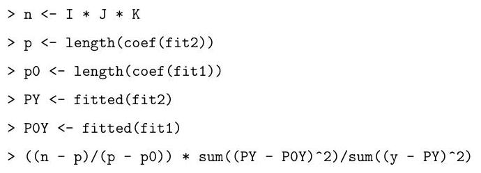
Finally, explain what is being calculated in the code below and give the value that would be obtained by the final line of code.


